* Aja Watkins is a PhD candidate at Boston University, but not for long. In the fall she will be starting a position as Assistant Professor of Philosophy at the University of Wisconsin, Madison. She writes…
A common refrain heard from climate scientists, policymakers, science journalists, and advocates, is that contemporary climate change is “unprecedented”—at least in certain respects and over certain timescales. For example, the Intergovernmental Panel on Climate Change (IPCC), the primary body responsible for determining and disseminating the scientific consensus in climate science, often makes this kind of claim. In the Technical Summary of their most recent Assessment Report they say, “Multiple lines of evidence indicate the recent large-scale climatic changes are unprecedented in a multi-millennial context,” and that “Global surface temperatures are more likely than not unprecedented in the past 125,000 years.”

The 2019–2020 Australian bushfires viewed from space
Of course, the IPCC is careful to include the caveat that these features of contemporary climate change are unprecedented only when considering certain timescales. Journalists or other science communicators are often less careful, at least in their headlines. For example, referring to that same IPCC report, a headline from the Washington Post reads, “Humans have pushed the climate into ‘unprecedented’ territory, landmark U.N. report finds” and the news section of Science ran the headline, “Climate change ‘unequivocal’ and ‘unprecedented,’ says new U.N. report.” We also frequently see headlines like, “The last 8 years were the hottest on record.” The word choice is a bit sneaky here, because “on record” really just means “since humans started measuring the global temperature” (the graphic in this New York Times piece goes back to 1940), but the claim sounds much grander than that. The word “unprecedented” is also often applied to other climate-change related phenomena, such as severe weather events (e.g., heat waves).
Those of us who are interested in the historical sciences like paleontology or, more relevant in this case, paleoclimatology should be automatically suspicious of the claim that contemporary climate change is unprecedented. Spoiler alert: it is also really hard to compare data about past and present climate change (like it is very hard to compare past and present data about biodiversity).
Although “as a matter of principle, earth history does not repeat itself” (Rosol 2015, 44)—so, of course, nothing exactly like contemporary climate change has ever happened before—Earth’s history is very long and contains very many climate fluctuations. It would be surprising, then, if Earth’s climate had really never before undergone the kinds of changes that it’s currently experiencing, or at least something fairly similar. The good news is that if there are past episodes of climate change that resemble contemporary climate change in certain relevant respects (increased atmospheric concentrations of carbon dioxide, warming, ocean acidification), we can potentially use these past sources of climate change as an important source of evidence to help us predict how contemporary climate change is going to play out. Such periods are sometimes called “paleoclimate analogues.”
The bad news is that the claim “contemporary climate change is unprecedented” has played an important rhetorical role in public discourse about climate change. Specifically, climate science deniers or skeptics have often tried to invoke the fact that Earth’s climate has changed many times before as a reason to think that contemporary climate change is no big deal. The scientists (among others) have responded by emphasizing the ways in which contemporary climate change is notably different from anything that has happened before. If we instead shift attention to the ways in which Earth’s history perhaps contains many climate episodes similar to that currently underway, we might have to give up on this particular response to the skeptics. (Luckily, there are many other responses available to us: for example, that any of these past climate change episodes would have been really bad for whatever organisms were around at the time, or that no climate episode like the current one has happened since the evolution of our species.)
Perhaps for these political or rhetorical reasons, even paleoclimatologists tend to call contemporary climate change “unprecedented.” In particular, they often claim that contemporary rates of climate change are unprecedentedly high, perhaps even in the entire geological past. For example, a statement by the Geological Society of London, in which they advocate for the use of paleoclimate analogues as a source of evidence about contemporary climate change, nonetheless says, “whilst atmospheric CO2 concentrations have varied dramatically during the geological past due to natural processes, and have often been higher than today, the current rate of CO2 (and therefore temperature) change is unprecedented in almost the entire geological past” (Lear et al. 2021, 1; for similar claims see National Research Council 2012 and Tierney et al. 2020). If contemporary rates of climate change are unprecedented, this may limit our ability to use paleoclimate analogues as a source of evidence about the predicted trajectory of and response to contemporary climate change. For instance, we have good reason to believe that the biotic response to climate change (adaptation, migration, extinction) is rate-dependent (e.g., Quintero and Wiens 2013). If rates between the past and present are always disanalogous, we might not be able to use paleoclimate analogues to inform our predictions about biotic response.
As it turns out, comparing rates of climate change in the deep past and today is really hard. One reason for this is that the data that we have about the deep past look very different than the data we have today. We measure past episodes of climate change using what are called “paleoclimate proxies,” such as ice cores, tree rings, sediment cores, and more, whereas we measure the climate today using very different techniques, such as thermometers at weather stations or satellite images. More importantly, while contemporary climate data are collected annually (or even more often), data about the deep past are collected at a much lower temporal resolution, sometimes with each data point only every several thousand years.
The implications of this difference in temporal resolution are profound, namely because the measured rates of a process (at least sometimes) depend systematically on the durations over which those rates are measured. More specifically, if you measure rates using long durations (a relatively low temporal resolution, like in the historical case), you will find systematically lower rates than if you measure rates using smaller durations (a relatively high temporal resolution, like in the contemporary case). Let me first try to convince you that this relationship really holds—it would be unsurprising if this is the first you’re hearing of it!—and then I’ll say more about what it means for determining whether contemporary rates of climate change are really unprecedented.
The easiest way to understand this relationship between rates and the durations over which they are measured is to use a more intuitive analogy: the relationship between the perimeter of irregular shapes—the standard example is usually the island of Great Britain—and the length of the measuring “stick” used to measure those perimeters. For shapes like these, which have outlines that are zig-zaggy, if you use a longer measuring stick you will get a shorter perimeter and if you use a smaller measuring stick you will get a longer perimeter. The relationship between length of measuring stick and perimeter leads to what is commonly called the “coastline paradox.” The word “paradox” in this context is used to describe the fact that if you decrease the length of your measuring stick infinitely, shapes like Great Britain will have an infinitely long perimeter. Furthermore, all such shapes (e.g., Australia) will have equally infinite perimeters.

The influence of ruler length on coastline measurement; with a longer “ruler: (left), the measured coastline is significantly shorter than that measured by a shorter “ruler” (right)
Just as the length of a perimeter of irregular shapes depends on the length of the measuring stick used to measure it, the rate of a process with a lot of “ups and downs” depends on the duration over which those rates are measured. Using smaller durations will yield higher rates, and vice versa. This relationship was first noticed in the context of sedimentology (Sadler 1981). Total accumulated sediment goes “up and down” as both sedimentation and erosion affect the remaining amount of sediment over time.
Here are some made up sedimentation data that I’ll analyze in order to convince you that this relationship between rates and durations actually holds for a process like this.

We can plot these data with time on the x-axis and accumulated sediment depth on the y-axis. Notice that the process has these “ups and downs” (because I concocted the example that way).

We can calculate a rate using any two of these data points. These rates correspond to different durations over which they were measured. We can now look at the relationship between rates and durations by plotting these rate data on a new graph: this time with durations on the x-axis and rates measured over those durations on the y-axis. I’ve included a line connecting the average rate for each duration in order to show you that we can start to see that the relationship between rates and durations exponentially decays—as durations increase, rates decrease exponentially.

The relationship is even clearer when we re-plot the data on a graph with the log of the durations on the x-axis and the log of the rates on the y-axis. Performing this conversion onto a log-log graph allows us to include a linear best-fit line for the data, and once we have a linear best fit line we are really in business, mathematically speaking. For example, it is very easy to calculate the slope of a linear best fit line. Notice that the slope of this best fit line is negative, such that higher durations produce lower rates.

The most important part about this best-fit line is that we can use it to extrapolate to the left and right of our rate data, or interpolate between the data points we already have, to figure out what the rate of the sedimentation process would have been if we had measured it over durations other than the ones we actually used. In other words, we can adjust our rate data to a higher or lower temporal resolution. This process of adjusting rates is called “temporal scaling”—we are scaling the rates to what they would have been if we had measured them differently. Crucially, if you want to compare rates of two different processes (say, sedimentation in two locations), you have to scale the rates to the same durations, even if the data weren’t originally gathered at similar temporal resolutions. Temporal scaling makes these comparisons possible and meaningful.
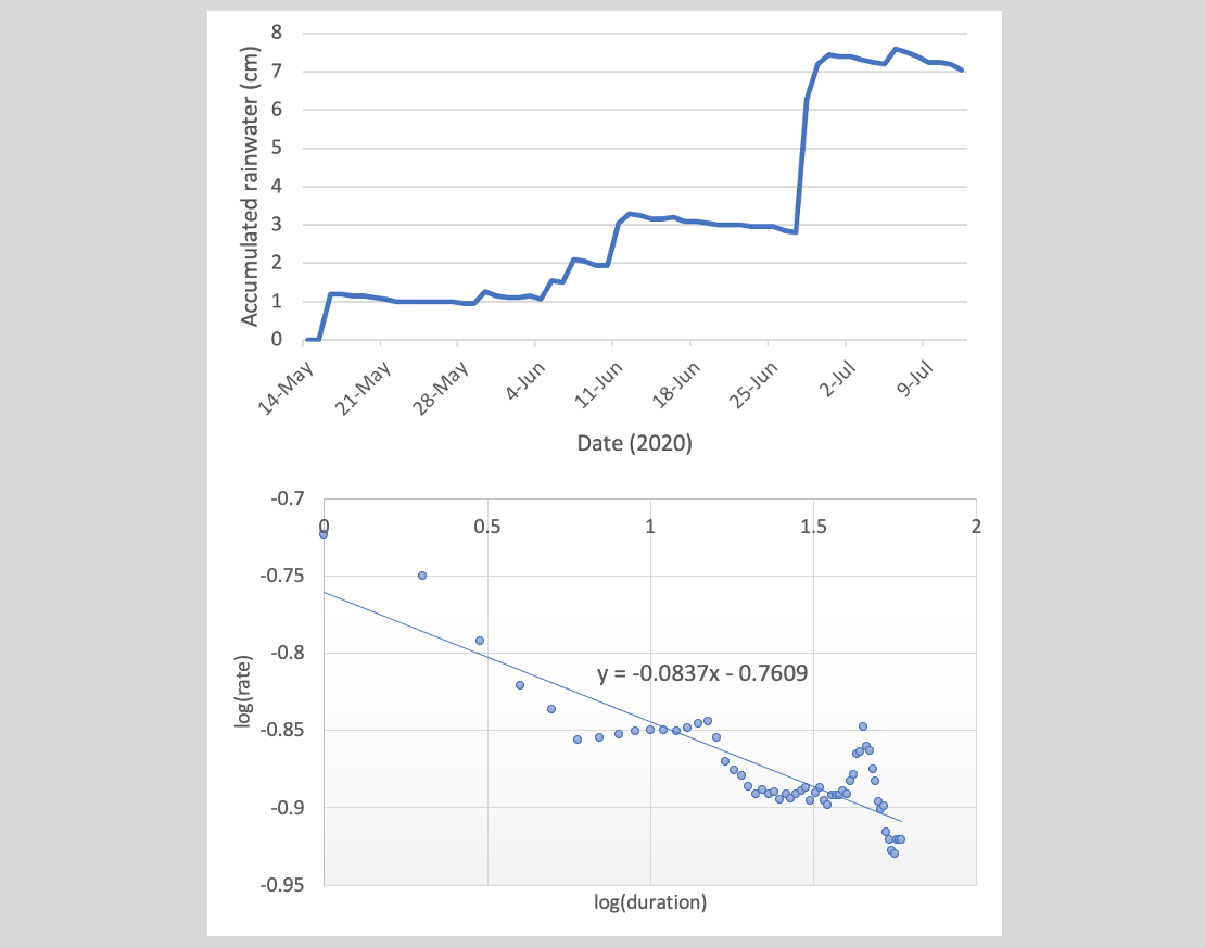
The inverse relationship between rates and the durations over which they are measured also holds in real-world cases as well. In the very boring summer of 2020, I decided to collect some rudimentary rain gauge data, just to convince myself that this relationship between rates and durations actually holds. If you don’t ever dump out a rain gauge, the water level in it will naturally go up and down, as both precipitation and evaporation occur. In Massachusetts, where I live, precipitation happens more quickly than evaporation does, so rainwater will accumulate gradually over time, although the process still exhibits some ups and downs. In New Mexico, where I grew up, evaporation generally happens faster than precipitation, so you end up with a lot of days with an empty rain gauge. (My father, who still lives in Albuquerque, collected some rain gauge data, too, and indeed found that his rain gauge was mostly empty, even shortly after it had rained. Thanks, Dad!) In either case, you’ll find that rates of accumulated rainfall and the durations over which those rates were measured have this negatively-sloped relationship on a log-log plot, like we saw in the fake sedimentation data above.
Temporal scaling is especially useful in the historical sciences because these are sciences where data are generally gathered at low and widely ranging temporal resolutions. For example, temporal scaling has been used to look at rates of evolution and extinction, in addition to rates of sedimentation. (In case anyone is interested in a juicy debate, Philip Gingerich used temporal scaling to argue that Niles Eldredge and Stephen Jay Gould’s theory of punctuated equilibria was wrong—he argued that their fast or slow rates of evolutionary change were just an artifact of the temporal resolutions at which those data were collected. They had a very lively back-and-forth on this topic in the ‘80s.)
Lo and behold, temporal scaling is useful in the context of paleoclimatology as well. Climate variables like temperature go up and down over long periods of time; this is a good indication that the rates of climate change will depend on the durations over which they are measured. For example, Kemp et al. (2015) found that rates of temperature change scale as predicted with durations for several past climate change episodes.

We can use temporal scaling in order to more meaningfully compare rates of climate change in the past to those in the present. If we don’t scale these rates to be as though they were measured over similar durations, it is very likely that the rates in the past will seem lower than in the present. But this would just be a feature of the fact that data about the past is generally at a much lower temporal resolution than data about the present. In order to determine the relationship between past and present rates, we need to adjust the data for this difference.
For example, Gingerich (2019)—yes, the same Gingerich—applied temporal scaling to rates of carbon accumulation during one candidate paleoclimate analogue, the Paleocene-Eocene Thermal Maximum (PETM), a major warming episode that took place about 55 million years ago. Indeed, the expected relationship between rates and durations holds in this case (see graph “a”).

Contemporary data, by contrast, don’t have this negatively-sloped relationship between rates and durations (graph “b”). That’s because contemporary emissions don’t have this up-and-down characteristic (they just go up, at least so far—over long enough periods of time, natural processes that draw carbon down out of the atmosphere will kick in). So, the relationship between rates and durations in the contemporary case shows a near-zero slope on that same log-log graph.
What does this mean about the relationship between rates of climate change in the deep past and how they compare to rates of climate change today? Unfortunately, not much. The problem is that we still haven’t specified which durations we should scale the rates to in order to compare them. For example, if we place the horizontal line representing contemporary climate change and the negatively-sloped line representing the PETM (or, frankly, any past climate episode) on the same graph, we will see that these lines are guaranteed to intersect somewhere. Consequently, there will be some durations for which it looks like past rates of climate change are higher than those in the present (smaller durations), one duration for which it looks like the past rates of climate change are the same as those in the present (where the lines intersect), and some other durations for which it looks like past rates of climate change are lower than those in the present (longer durations). What are we to do? How should we decide over what durations to compare the rates?

I have a few ideas about how to solve this problem. First, notice that the line representing the past event is subject to a lot of uncertainty. We will have collected data about the past climate episode over a particular set of durations, likely rather high durations. As the best fit line gets extrapolated further and further away from the data we’ve actually collected, the line becomes less tightly constrained, i.e., the uncertainties increase. At some point—I’m not sure exactly where—the degree of uncertainty will become unacceptable to the scientists working on this. The amount of acceptable uncertainty can be used to set an upper and lower bound on the range of acceptable durations to use.
Second, the duration of an event itself can be used to set an upper bound on the range of acceptable durations. For example, the PETM didn’t last forever (about 100,000 years), so it doesn’t make sense to extrapolate to longer durations than the PETM actually lasted. Likewise, the contemporary climate episode won’t last forever either—most probably, much less long than the PETM—so it doesn’t make sense to extrapolate that horizontal line out to the right forever, either. The durations over which we compare these rates must be durations that make sense given how long the relevant events themselves lasted.
Third, I think it’s possible that researchers may be able to further constrain the range of acceptable durations by considering the purposes for which we want to use the paleoclimate analogue. For instance, if we want to use the paleoclimate analogue to make predictions over 100-500 year timescales, we better be comparing past and present rates over durations of 100-500 years. In case anyone is interested, PETM rates are the same as contemporary rates over a duration of about 178 years, according to the data Gingerich used.
Applying these three constraints on the range of acceptable durations might either yield inconsistent upper and lower bounds (an empty set of acceptable durations) or tell us that a past climate episode has very different (higher or lower!) rates than contemporary climate change, in which case maybe we are no longer interested in using that past episode as an analogue. But it might also tell us that past and present climate change episodes weren’t so different after all, with respect to rates. If so, we might be able to use the past climate episode to inform our predictions about contemporary climate change, even for rate-dependent processes like biotic response. However, it is important to also make predictions over the same durations we used to establish analogy between the past and present climate episode—if we make predictions over different durations than that, we’ll be making predictions over durations for which we know that the past and present climate episode occurred at different rates, exactly what we’ve been trying to avoid.
We’ve now seen that comparing rates of climate change in the deep past to those today is really complicated, and we are left without a definitive answer about whether contemporary rates of climate change are unprecedented, because what these rates are depends on how we choose to measure them. Interestingly, whether we take past rates to be higher, lower, or the same as contemporary rates depends in part on what our research purposes are, since these inform which durations we use to compare the rates.
I want to close with two other, philosophically relevant points about rates. Here’s the first: What are the “real” rates of processes like climate change, if the measured rate depends on the duration we use? I think there are a few ways to go here. First, one might specify a specific, salient duration over which to measure the rates, and claim that all rates of that kind of process should be scaled to that duration, over which we will find the “real” rate of that process. (Gingerich argued we could do this for evolutionary rates, which he thought should all be scaled to a duration of one generation.) The problem with this view is that it’s unclear what this salient duration would be for many processes, like climate change. Second, we might say that more precise measurements are always better, and that we should look at what the rate would be as the duration approaches one that is infinitesimally small. The problem here is that all rates that had this inverse relationship with durations—rates of sedimentation, precipitation, evolution, climate change—would then be “really” infinitely high. Recall that in the context of measuring perimeters of coastlines, noticing that the perimeters approach infinity as we use shorter and shorter measuring sticks is what generates the coastline paradox.
A third way to go is to say that there aren’t “real” rates of change for these processes. This view accords with what fractal geometer Benoit Mandelbrot (namesake of the Mandelbrot set fractal) thought about perimeters. He said that the length of a coastline “turns out to be an elusive notion that slips between the fingers of one who wants to grasp it” (Mandelbrot 1982, 25). The idea here is that maybe there isn’t a true perimeter of Great Britain; the perimeter just depends on how we choose to measure it. Similarly, maybe there isn’t one true rate for processes that have this fractal quality; the rate just depends on how we decide to measure (or scale) it. And that might, in turn, depend on our research purposes.
Here is the second point: I’ve been taking for granted that we can carve up the history of Earth’s climate into specific events, like the PETM or contemporary climate change. However, there is some dispute among historical scientists about how, exactly, to demarcate events. The problem is that sometimes events are demarcated by (what seem to be) notable rates. But, again, rates depend on the durations over which they are measured, so it isn’t straightforward to say what rate these processes “really” happened at during the relevant periods of time. Take the case of mass extinctions for example. It isn’t clear what makes an extinction event count as a mass extinction (Bocchi et al. 2022), but one view is that mass extinctions are distinguishable by particularly high rates of extinction. We can now see that this isn’t going to work—biodiversity has these up and down fluctuations that indicate the need to adjust rates by durations, but it isn’t necessarily clear what durations to use in scaling extinction/origination rates, and so it is difficult to tell what the “real” rate of extinction is in any given period of time. We may have other ways of demarcating mass extinction events (e.g., based on magnitude or cause of the extinctions), but it would be ill-advised to rely on rates to do so.
References
Bocchi, F., Bokulich, A., Castillo Brache, L., Grand-Pierre, G., Watkins, A. 2022. Are we in a sixth mass extinction? The challenges of answering and value of asking. The British Journal for the Philosophy of Science. https://doi.org/10.1086/722107
Gingerich, P.D. 2019. Temporal scaling of carbon emission and accumulation rates: modern Anthropogenic emissions compared to estimates of PETM onset accumulation. Paleoceanography and Paleoclimatology 34:329–335. https://doi.org/10.1029/2018PA003379
Kemp, D.B., Eichenseer, K., Kiessling, W. 2015. Maximum rates of climate change are systematically underestimated in the geological record. Nature Communications 6:8890. https://doi.org/10.1038/ncomms9890
Lear, C. H., Anand, P., et al. 2021. Geological Society of London Scientific Statement: What the geological record tells us about our present and future climate. Journal of the Geological Society 178. https://doi.org/10.1144/jgs2020-239
Mandelbrot, B.B. 1982. The Fractal Geometry of Nature. W.H. Freeman and Co.
National Research Council. 2012. Understanding Earth’s Deep Past: Lessons for our Climate Future (Vol. 49).
Quintero, I., Wiens, J.J. 2013. Rates of projected climate change dramatically exceed past rates of climatic niche evolution among vertebrate species. Ecology Letters 16:1095–1103. https://doi.org/10.1111/ele.12144
Rosol, C. 2015. Hauling data: Anthropocene analogues, paleoceanography and missing paradigm shifts. Historical Social Research 40:37–66. https://doi.org/10.12759/hsr.40.2015.2.37-66
Sadler, P.M. 1981. Sediment accumulation rates and the completeness of stratigraphic sections. The Journal of Geology 89:569–584. https://doi.org/10.1086/628623
Tierney, J.E., Poulsen, C.J., Montañez, et al. 2020. Past climates inform our future. Science 370. https://doi.org/10.1126/science.aay3701